What breed is that puppy? Dog breed classification using Convolutional Neural Networks and Transfer Learning in Keras

In what follows I’ll show how to build a computer vision application with Keras and Tensorflow for classifying dog images according to their breed. The presented model focuses on two particular breeds, Chihuahua and Pug, and relies on Convolutional Neural Networks, a state-of-art deep learning model for the image classification task.

Convolutional Neural Networks

Convolutional neural networks (CNNs) are a deep learning model inspired by the organization and functioning of the animal visual cortex. Individual neurons are arranged so as to respond to partially overlapping regions that make up the visual field, called receptive fields. These networks can learn a meaningful representation of a given image by automating the feature extraction process. The classical architecture of a CNN consists of a series of particular layers:

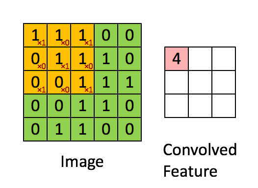
• Convolutional layer: given an input image the convolution is carried out using a set of filters, called kernels, which are matrices of learnable weights. Convolution is performed using dot product between the filter and the portion of the image over which it is hovering; the filter is shifted according to a stride parameter and this process is repeated until the the entire image has been covered, generating an output volume composed by a set of convolved feature maps. The convolution of a \(3\times 3\) kernel, with \(stride=1\) (one pixel at a time) applied to a single-channel \(5\times 5\) image is shown below:
• Relu layer: Rectified Linear Unit is the typical activation function of convolutional levels, defined as \(f(x) = max(0, x)\). This function has many interesting properties, including efficiency, robustness against weight saturation or vanishing gradient, as well as the sparse activation of artificial neurons, which mimics what happens in biological systems, where only few neurons activate simultaneously.
• Pooling layer: the role of this layer is to reduce the spatial size of the output volume from the convolutional layer, extracting rotational and positional invariant features. Dimensionality reduction is carried out using a kernel which moves upon the input matrices, taking the maximum (or the average) of the covered values.
• Fully-connected layer: the output of convolutional and pooling layers can be flattened and feed to a dense layer of fully connected neurons, in order to learn a non-linear combination of the learned features. Finally a softmax classifier can be used for determining a probability value for each class label.

Chihuahua vs. Pug

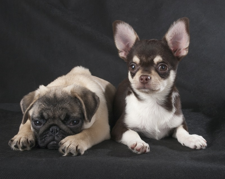
Let’s now move on how to use Convolutional Neural Networks in Keras in order to build our breed classifier, for distinguish a Chihuahua from a Pug. Our dataset is an extract from Dog Breed Identification, and is composed by 152 Chihuahua and 200 Pug images. Data are normalized and resized to a fixed shape of \(350\times 350\). Now let’s look at some example images from our dataset: 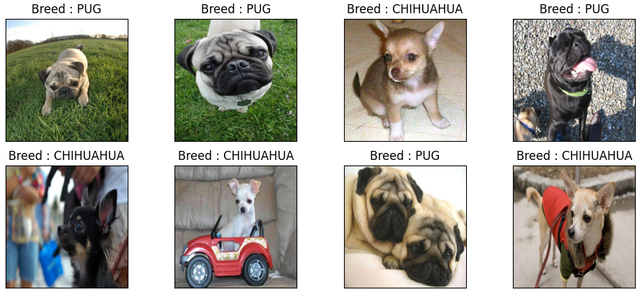This is a really challenging classification task, as the patterns to be learned are quite complex and the training images are few compared to how many a CNN would need to learn meaningful features. In order to cope with the small amount of traning data, the model exploits three main techniques:

• Transfer Learning
• Real time data augmentation
• Fine tuning

Transfer Learning

Transfer Learning technique consists of exploiting features learned on one problem, for dealing with a new similar problem: this way, the abilities of a pre-trained model can be transferred to another. This technique is very usefull when data are not enough to build a full model from scratch, as in our case. I exploited this strategy creating our dog breed classifier as follows:

• Load the pre-trained model: I used a VGG16 model which has been pre-trained on ImageNet, a +10 million image dataset from 1000 categories.
• Freeze VGG16 layers, so as to avoid destroying the information they contain during training.
• Add a multilayer perceptron on top of them, composed by two trainable fully connected layers, Dropout for preventing overfitting and a softmax classifier for determining the output probability for each class.

The Keras implementation of the model is shown below:

def transfer_learning():
    vgg_conv = vgg16.VGG16(weights='imagenet', include_top=False, input_shape=(350, 350, 3))
    for layer in vgg_conv.layers[:]:
        layer.trainable = False
    model = Sequential()
    model.add(vgg_conv)
    model.add(Flatten())
    model.add(Dense(1024, activation='relu'))
    model.add(Dropout(0.5))
    model.add(Dense(512, activation='relu'))
    model.add(Dropout(0.5))
    model.add(Dense(2, activation='softmax'))
    model.summary()
    return model

Training the model with real time data augmentation

Now our model is ready for the training step. As the amount of images available for training the model is small, we can use an ImageDataGenerator in order to obtain some additional training samples:

datagenTrain = ImageDataGenerator(
    featurewise_center=True,
    featurewise_std_normalization=True,
    rotation_range=20,
    width_shift_range=0.2,
    height_shift_range=0.2,
    horizontal_flip=True)
datagenTrain.fit(xTrain)

Now we can use our generator while training the model, obtaining real time data augmentation:

# compile model
model.compile(loss='categorical_crossentropy', optimizer="adam", metrics=['accuracy'])
# set callbacks for early stopping
es = EarlyStopping(monitor='val_loss', mode='min', verbose=1, patience=5)
best_weights_file = "weights.h5"
mc = ModelCheckpoint(best_weights_file, monitor='val_loss', mode='min', verbose=2,
                     save_best_only=True)
# train model testing it on each epoch with real time data augmentation
history = model.fit(datagenTrain.flow(xTrain, y_train_cat, save_to_dir= "data_aug", batch_size=32), validation_data=(xTest, y_test_cat),
                    batch_size=32, callbacks= [es, mc], epochs=50, verbose=2)

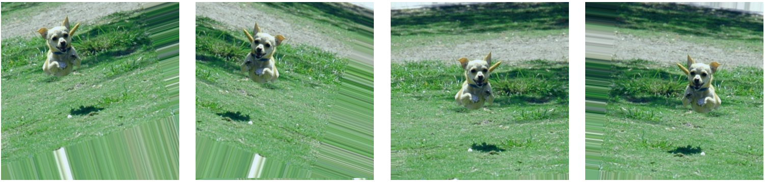
An example of what images our generator produces, using 20° rotation, shift and horizontal flip, is shown below: The model has been trained using the categorical crossentropy loss function and the Adam optimizer. Furthermore two callback functions have been used in oder to avoid overfitting: EarlyStopping, which monitors the loss on validation set, and ModelCheckpoint for storing the best model.

Fine tuning

An additional step for further improving performances is fine tuning. It consists in re-training the entire model obtained above in order to incrementally adapt the pretrained features to our specific dataset. Specifically, fine tuning can be obtained as follows:

• Load the best model achieved in the previous training step
• Un-freeze the pretrained layers. I’ve choosen to make the entire model trainable for a full end-to-end tuning.
• Compile the model.
• Train it with a very low learning rate. It’s crucial to set a low learing rate as we only want to readapt pretrained features to work with our dataset and therefore large weight updates are not desirable at this stage.

The code is shown below:

model.load_weights(best_weights_file) # load the best model saved by ModelCheckpoint
model.trainable = True
best_weights_file = "weights_fine_tuned.h5"
mc = ModelCheckpoint(best_weights_file, monitor='val_loss', mode='min', verbose=2,
                     save_best_only=True)
model.compile(loss='categorical_crossentropy', optimizer=Adam(1e-5), metrics=['accuracy'])
history = model.fit(datagenTrain.flow(xTrain, y_train_cat, batch_size=32), validation_data=(xTest, y_test_cat),
                    batch_size=32, callbacks= [es, mc], epochs=50, verbose=2)

Results

In order to analyze the benefits introduced by the use of Transfer Learning and fine tuning, I compared the model described above with a simple CNN, trained from scratch with data augmentation, whose structure is shown below:

def build_simple_CNN():
    model = Sequential()
    model.add(Conv2D(filters=32, kernel_size=(3,3),strides=(2,2), padding="valid",
                     activation="relu", input_shape=(IMG_SIZE,IMG_SIZE,CHANNELS)))
    model.add(MaxPooling2D(pool_size=(3,3),strides=(2,2)))
    model.add(BatchNormalization())
    model.add(Conv2D(filters=64,kernel_size=(3,3),strides=(2,2), padding="valid",
                     activation="relu"))
    model.add(Flatten())
    model.add(Dense(512, activation="relu"))
    model.add(Dropout(0.3))
    model.add(Dense(2, activation="softmax"))
    model.summary()
    return model

The following table shows a comparison between the performances achieved by the simple CNN and the proposed model:

	Accuracy	Precision	Recall	F1-Score
Simple CNN	0.68	0.70	0.68	0.64
Transfer Learning	0.87	0.88	0.87	0.87
Transfer Learning + Fine Tuning	0.93	0.93	0.93	0.93

As we can easily see, the use of Tranfer Learning has led to much higher performances than a simple Convolutional Neural Network trained from scratch (0.68 vs. 0.87 accuracy). In addition, the fine tuning step has further improved performance significantly, reaching a 0.93 accuracy on the test set.

Now let’s take a closer look at the output of the model given some test images.

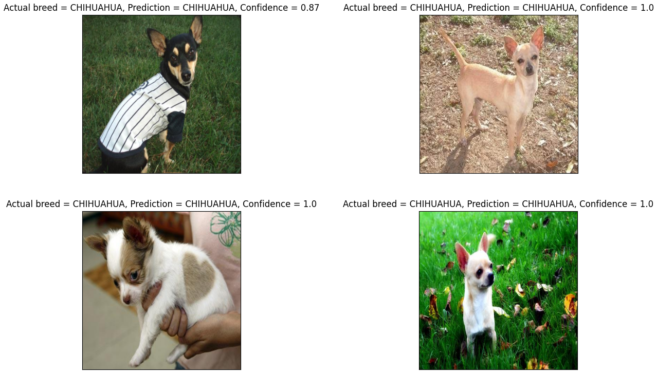
Chihuahua

Pug

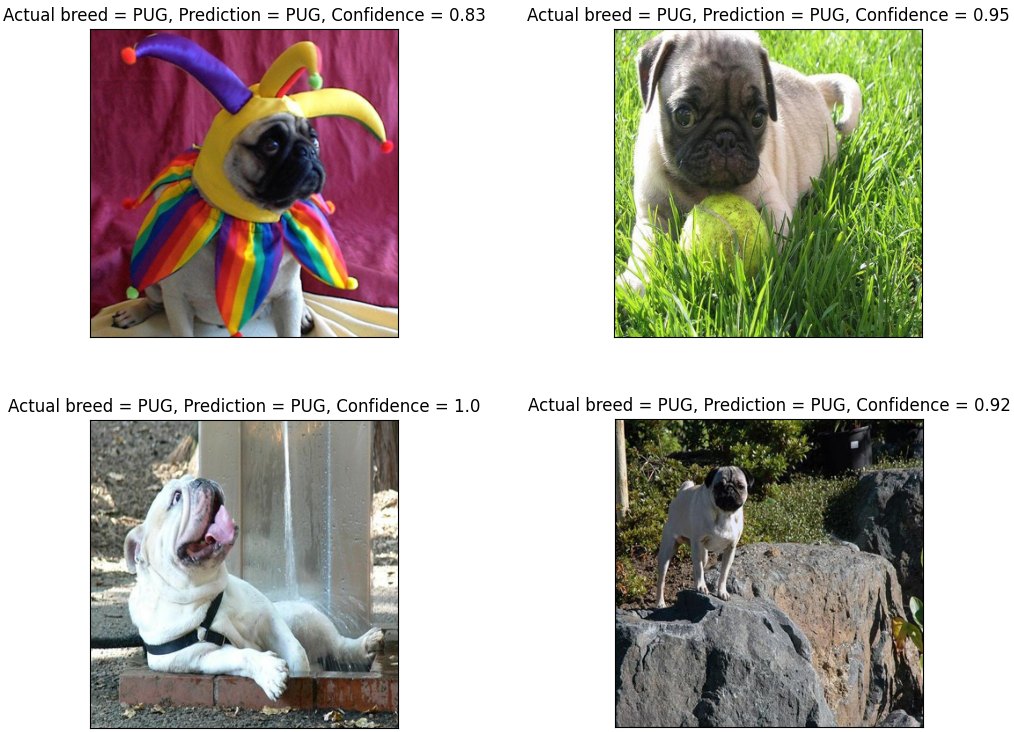Good job! The model is able to correctly classify dog images according to the breed with a high confidence level.

Special guest

Lastly, we can test our breed classifier with external images (this is the funniest part). To do this I took some photos of my girlfriend’s Chihuahua, Emy. Let’s see what our model says about this beautiful puppy: 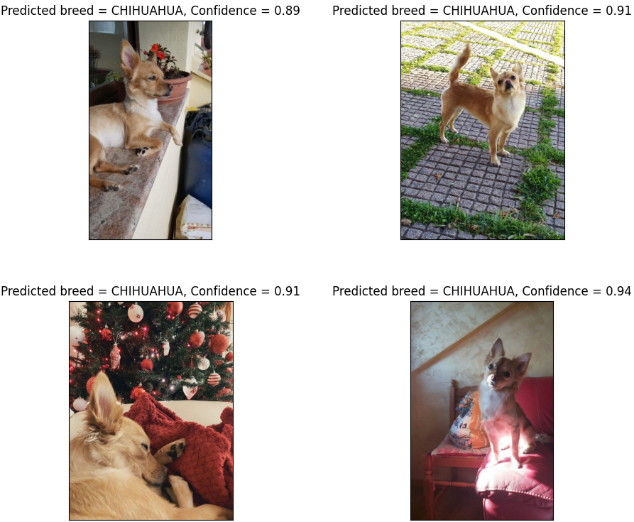Great! The model correctly classifies our cute Emy as a Chihuahua 👏👏

---

You can find the full code on GitHub at this link.